Hierachical aligner GC (or Hierarchical Clustering aligner)
Description
Feature list methods → Alignment → Hierachical aligner (GC)
This method aligns detected features in different samples through a match score. This score is calculated based on the mass spectrum and retention time of each peak and ranges of tolerance stipulated in the parameters setup dialog.
General Algorithm
This module uses the principles of agglomerative / hierarchical clustering approaches. The general principle behind those algorithms is described below.
Given a set of N items to be clustered, and an NN distance (or similarity) matrix, the basic process of hierarchical clustering* (defined by S.C. Johnson in 1967 - https://home.deib.polimi.it/matteucc/Clustering/tutorial_html/hierarchical.html#johnson) is this:
- Start by assigning each item to a cluster, so that if you have N items, you now have N clusters, each containing just one item. Let the distances (similarities) between the clusters the same as the distances (similarities) between the items they contain.
- Find the closest (most similar) pair of clusters and merge them into a single cluster, so that now you have one cluster less.
- Compute distances (similarities) between the new cluster and each of the old clusters.
- Repeat steps 2 and 3 until all items are clustered into a single cluster of size N. (*)
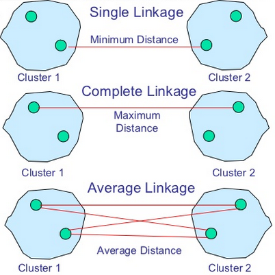
Step 3 can be done in different ways based on linkage criteria:
-
In single-linkage clustering (also called the connectedness or minimum method), we consider the distance between one cluster and another cluster to be equal to the shortest distance from any member of one cluster to any member of the other cluster. If the data consist of similarities, we consider the similarity between one cluster and another cluster to be equal to the greatest similarity from any member of one cluster to any member of the other cluster.
-
In complete-linkage clustering (also called the diameter or maximum method), we consider the distance between one cluster and another cluster to be equal to the greatest distance from any member of one cluster to any member of the other cluster.
-
In average-linkage clustering, we consider the distance between one cluster and another cluster to be equal to the average distance from any member of one cluster to any member of the other cluster.
A variation on average-link clustering is the UCLUS method of R. D'Andrade (1978) - https://home.deib.polimi.it/matteucc/Clustering/tutorial_html/hierarchical.html#dandrade - which uses the median distance, which is much more outlier-proof than the average distance.
All implemented types of hierarchical clustering are called agglomerative because they merge clusters iteratively. There is also a divisive hierarchical clustering, which does the reverse by starting with all objects in one cluster and subdividing them into smaller pieces. Divisive methods are not generally available, and have rarely been applied.
Of course there is no point in having all the N items grouped in a single cluster. But, once you have got the complete hierarchical tree, if you want to change number of clusters to \(k\), you can just cut the \(k-1\) longest links.
Available linkage criteria
Several linkage criteria are available:
- Single
- Complete
- Average
A linkage criteria determines the distance between sets of observations as a function of the pairwise distances between observations.
Some commonly used linkage criteria between two sets of observations \(A\) and \(B\) are:
| Name | Description |
|---|---|
| Maximum or complete-linkage clustering | \(max \{ d(a,b):a \in A, b \in B \}\) |
| Minimum or single-linkage clustering | \(min \{ d(a,b):a \in A, b \in B \}\) |
| Mean or average-linkage clustering, or UPGMA | \(\frac{1}{\lvert {A} \rvert \lvert {B} \rvert} \sum_{a \in A} \sum_{b \in B} d(a,b)\) |
where \(d\) is the chosen metric.
MZmine GC: Specific considerations
To obtain a distance matrix between all pairs of observations:
- A similarity score based on chemical likelihood only (chemSimScore) is computed.
Calculation of the dot product is based on work by [Stein and Scott (1994)](https://link.springer.com/article/10.1016/1044-0305(94)87009-8), which is the most popular approach for spectrum similarity measure.
Between two mass spectra $I_{t_j}$ and $I_{r_i}$ of two peaks $t_j$ and $r_i$ similarity is calculated as follows:

$$S(t_j,r_i)=dot(I_{t_j},I_{r_i})=<I_{t_j},I_{r_i}>/ (\lvert I_{t_j} \rvert \lvert I_{r_i} \rvert)$$
-
Then a similarity score based on RT likelihood only (rtScore) is computed.
Retention time score is normalized relatively to the RT window tolerance provided by the user
\[rtScore=\frac{1.0 d-rtDiff}{rtMaxDiff}\] -
A combined weighted (or mixture) score is determined based on a mixture of the above two scores
The final mixture score
\[score = (chemSimScore * mzWeight) + (rtScore * rtWeight))\]
A final square matrix is generated by comparing all the scores, for all the pairs of peaks.
Getting clusters from rooted binary tree
The algorithm methods described above all lead to a unique binary tree where all items are clustered into a single cluster of size N (number of leafs).
One more step is required to get the very final clusters list. A "cutoff" based on two criterion allows to split the single cluster into appropriate subgroups:
- A cluster cannot contain more than one leaf per sample
- A cluster cannot contain two leafs for which the distance (or mixture similarity score) is too low
Method parameters
Clustering strategy
What strategy will be used for the clustering algorithm decision-making.
Feature list name
Name of the new aligned peak list.
m/z tolerance
This value sets the range, in terms of m/z, for possible peaks to be aligned. Maximum allowed m/z difference.
Weight for m/z
The assigned weight for m/z difference at the moment of match score calculation between feature rows. In case of perfectly matching m/z values the score receives the complete weight.
Retention time tolerance
Maximum allowed difference between two RT values.
Weight for RT
The assigned weight for RT difference at the moment of match score calculation between peak rows. In case of perfectly matching RT values the score receives the complete weight.
Export dendrogram as TXT/CDT
If checked, exports the resulting dendrogram to the given *txt file.
Dendrogram output text filename
Name of the resulting TXT file to write the clustering resulting dendrogram to. If the file already exists, it will be overwritten.